Merkle trees are widely used in cryptography for data integrity and verification. Appendix E of the Gray Paper provides formal definitions for different types of Merkle trees, including the well-balanced Merkle tree, constant-depth Merkle tree, and Merkle Mountain Range. This article explains these concepts, along with the trace operator used for generating Merkle proofs. The node operator is introduced as a foundational structure to highlight similarities between well-balanced and constant-depth Merkle trees.

Node Operator:

The node operator is a generalized binary Merkle tree where each branch node has at most one more element on the left side than the right side. By "element," we refer to input elements, which is not the same as a leaf which can be the "hash zero" sometimes. The hash computations are as follows:

• For a branch node:

where node is the byte array of the string "node" in UTF-8, and ∼ is the append bytes operator.

Example:

• Input values [0, 1, 2, 3, 4, 5, 6, 7, 8] are divided using upper floor math of 9/2, resulting in 5 elements on the left and 4 on the right, repeated recursively.

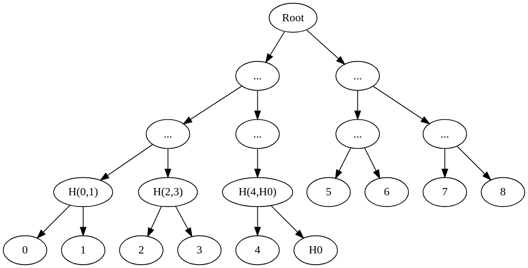
• Input values [0, 1, 2, 3, 4, 5, 6, 7, 8, 9, 10, 11, 12] are divided using upper floor math of 13/2, resulting in 7 elements on the left and 6 on the right, repeated recursively.

Well-Balanced Merkle Tree:

A well-balanced Merkle tree is similar to the node operator in that each branch node has at most one more element on the left side than on the right, with "element" referring to input elements. Some leaves may represent "hash zero" when no sibling leaf exists. The second key feature of the well-balanced merkle tree is that the depth difference between any two leaves is at most one.

• For a leaf v:

• For a branch:

where node is the byte array of the string "node" in UTF-8, and ∼ is the append bytes operator.

Example:

• Input values [0, 1, 2, 3, 4, 5, 6, 7, 8] are divided using upper floor math of 9/2, resulting in 5 elements on the left and 4 on the right, repeated recursively.

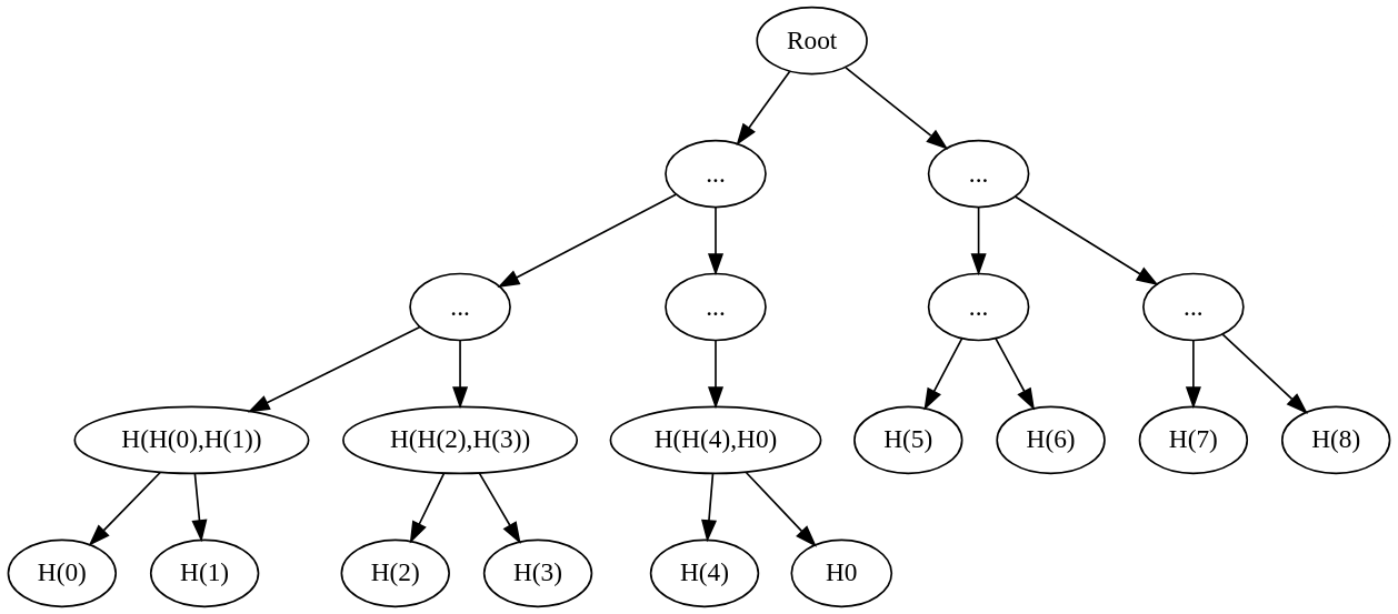
• Input values [0, 1, 2, 3, 4, 5, 6, 7, 8, 9, 10, 11, 12] are divided using upper floor math of 13/2, resulting in 7 elements on the left and 6 on the right, repeated recursively.

Constant-Depth Merkle Tree:

A constant-depth Merkle tree ensures that the tree has uniform depth by padding with "hash zero" to make the number of leaves a power of two. This guarantees that both sides of the tree have an equal number of leaves, which simplifies certain cryptographic operations.

• For a leaf v:

• For a branch:

where node is the byte array of the string "node" in UTF-8, and leaf is the byte array of the string "leaf" in UTF-8.

Example:

• Input values [0, 1, 2, 3, 4, 5, 6, 7, 8] are padded with zeros to make the length a power of two, resulting in [0, 1, 2, 3, 4, 5, 6, 7, 8, 0, 0, 0, 0, 0, 0, 0]. These are divided into two equal sets.

• Input values [0, 1, 2, 3, 4, 5, 6, 7, 8, 9, 10, 11, 12] are padded with zeros to make the length a power of two, resulting in [0, 1, 2, 3, 4, 5, 6, 7, 8, 9, 10, 11, 12, 0, 0, 0]. These are divided into two equal sets.

Trace Operator (Merkle Proof):

The trace operator is used to navigate the Merkle tree and generate a proof for a specific input element v at index i. The proof is constructed by iterating over the tree and, at each level, adding the opposite side’s hash to the proof set. We then recurse on the side of the tree containing the index i (left or right) and update i accordingly until reaching the leaf.

• Provides the set of elements from the opposite side of i. That is elements on the right side if i is on the right, and elements on the left side if i is on the left.

• Provides the set of elements (left or right) that contain the element at index i for generating the proof.

• Provides the index of the element within the recursive set (left or right).

Here’s how the process is formalized without using math notation:

• 1. At each level of the tree, we first identify the side containing the element we are generating a proof for (either the left or right side of the tree based on the element's index).
• 2. We then add the opposite side's hash to the proof.
• 3. After adding the hash of the opposite side to the proof, we update the index iii recursively. The new index is calculated by removing the portion of the array that doesn't contain the element. This means we reduce the index by the number of elements on the opposite side, essentially moving deeper into the tree with the updated index. This process is repeated until we reach the leaf level.

Example for a constant-depth Merkle tree:

Let’s take the input elements [0, 1, 2, 3, 4, 5, 6, 7, 8, 9, 10, 11, 12], padded to a power of two as [0, 1, 2, 3, 4, 5, 6, 7, 8, 9, 10, 11, 12, 0, 0, 0]. We want to generate a proof for the element at index 9.

First Level:

• The input elements are split into two sets: [0, 1, 2, 3, 4, 5, 6, 7] on the left and [8, 9, 10, 11, 12, 0, 0, 0] on the right.
• Since the element at index 9 is in the right set, we add the hash of the left set (let's call it Ha​) to the proof.
• The proof is now [Ha​].
• The index is updated by subtracting the number of elements in the left set (which is 8), so the new index becomes 1.

Second Level:

• We now have the right set [8, 9, 10, 11, 12, 0, 0, 0], which is split into two sets: [8, 9, 10, 11] on the left and [12, 0, 0, 0] on the right.
• Since the element at index 1 is in the left set, we add the hash of the right set (let's call it Hb​) to the proof.
• The proof becomes [Ha, Hb​].
• The index is updated again, but this time by subtracting the number of elements in the left set (which is 0), so the new index remains 1.

Third Level:

• The left set is now [8, 9, 10, 11], which is split into [8, 9] on the left and [10, 11] on the right.
• Since the element at index 1 is in the left set, we add the hash of the right set (let's call it Hc) to the proof.
• The proof becomes [Ha​, Hb​, Hc​].
• The index is updated by subtracting 0, so the new index remains 1.

Final Level:

• The left set is now [8, 9]. Since the element at index 1 is in this set, we add the hash of the opposite element [8] to the proof. This completes the proof since we have reached the leaf level.
• The final proof is [Ha, Hb​, Hc​, H(10,11)].

Merkle Mountain Range (MMR)

The Merkle Mountain Range (MMR) is an append-only cryptographic data structure that enables efficient commitment to a sequence of values. It allows for constant-time (logarithmic) appending and proof generation for inclusion within the structure, making it scalable even as the dataset grows.

Key Properties of the MMR:

• Append-Only: Once a value is appended to the MMR, it cannot be removed or modified.
• Efficiency: Both appending to the MMR and generating proofs of inclusion are O(log⁡(N))O(\log(N))O(log(N)) in time and space, where NNN is the size of the set.
• Peaks and Merkle Trees: The MMR consists of a series of peaks, each representing the root of a Merkle tree. The number of elements in each peak corresponds to powers of two (i.e., 2i2^i2i, where iii is the index in the sequence). For non-power-of-two sequences, some peaks may be empty.
• Commitment: To commit to the entire sequence, the MMR is typically hashed. Once hashed, no further appending is allowed, and the commitment serves as the "snapshot" of the data at that point.

Walk-Through Example: Appending Elements to an MMR

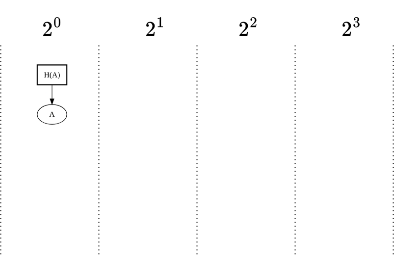
Step 1: First Element (A)

• Initial State: The MMR is empty.
• Append: We append element A.
• Result: Since this is the first element, it forms a single leaf in a new peak.

Step 2: Second Element (B)

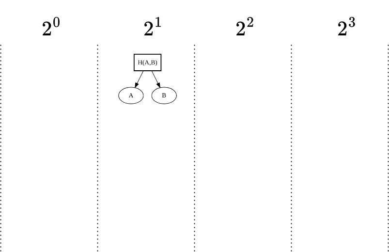
• Append: Now we append element BBB.
• Result: Elements A and B form a binary Merkle tree. The hash of A and B becomes the new root for this peak.

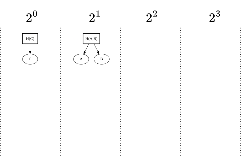
Step 3: Third Element (C)

• Append: We append element C.
• Result: Since C cannot merge with the existing peak (which is full), it becomes its own peak. The MMR now has two peaks.

Step 4: Fourth Element (D)

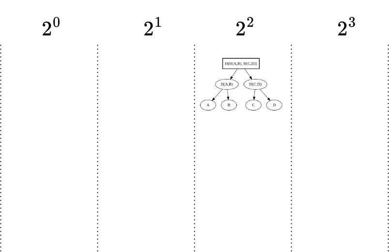
• Append: Now we append element D.
• Result: Elements C and D merge into a new Merkle tree. The MMR now has two peaks: one rooted in H(C,D) and the other rooted in H(A,B).

Step 5: Fifth Element (E)

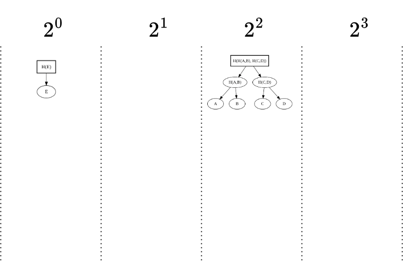
• Append: Element E is added.
• Result: Since no further merging is possible, E forms a new peak by itself. Now, we have three peaks.

Step 6: Sixth Element (F)

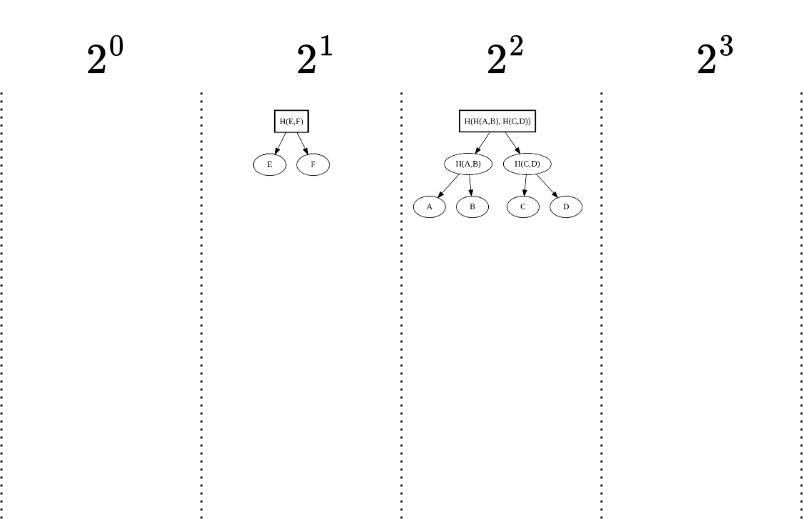
• Append: Now we append F.
• Result: Elements E and F merge into a new peak.

Step 7: Seventh Element (G)

• Append: We append element GGG.
• Result: Since there’s no other element to merge with, GGG remains a standalone peak.

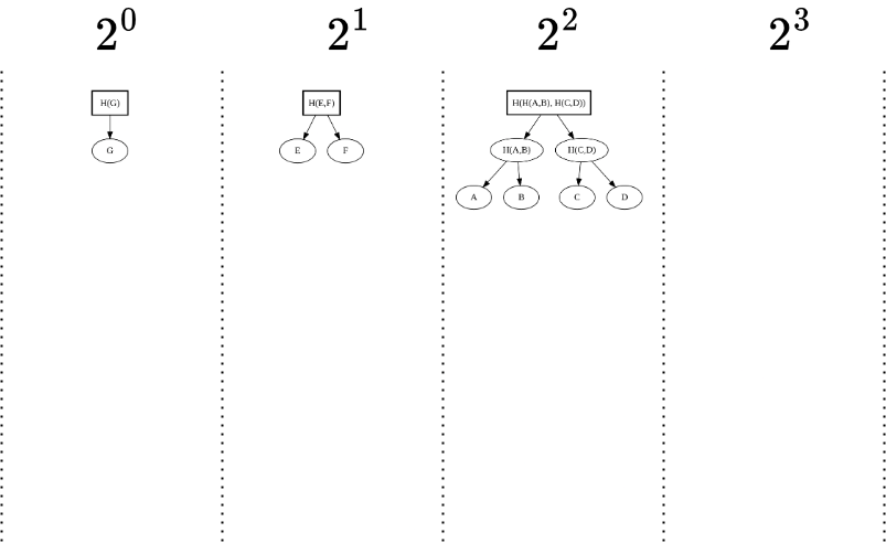
Step 8: Eighth Element (H)

• Append: Finally, we append element H to the Merkle Mountain Range (MMR).
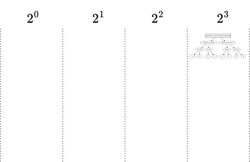
• Result: Element H merges with element G to form a new Merkle tree with root H(G,H).
• Now, we have two peaks at this stage:
  • Peak 1: A large Merkle tree rooted at H(H(A,B),H(C,D)), representing the first four elements (A,B,C,D).
  • Peak 2: A tree rooted at H(H(E,F),H(G,H)), representing the next four elements (E,F,G,H).
• Since we now have two peaks with the same height (both containing 2^2 =4 elements), these two trees will merge into one peak, combining the entire sequence of 8 elements.
• Final Merge:
  • Peak 1: H(H(A,B),H(C,D))H(H(A,B), H(C,D))H(H(A,B),H(C,D))
  • Peak 2: H(H(E,F),H(G,H))H(H(E,F), H(G,H))H(H(E,F),H(G,H))
  • These two peaks are merged to form a single root: H(H(H(A,B),H(C,D)),H(H(E,F),H(G,H)))

Exploring MMR:

If you want to play with the Merkle Mountain Range and see how it works in real-time, you can experiment with an MMR tool at the following link: MMR Drawer. However, please note that the tool uses right-to-left appending (opposite to our left-to-right approach in this explanation).